Terrain: One Mesh from Orbit to Contact
The terrain requirement is one sentence: fly from orbit to walking height with gradual, pop-free refinement. Mountains keep their shape while distant, approaching reveals ridges and gullies continuously, and landing is not followed by a twenty-second mountain-building event. This post is how that is built: the levels, the tile lookup, the mesh, the streaming, and the detail stack above the measured data.
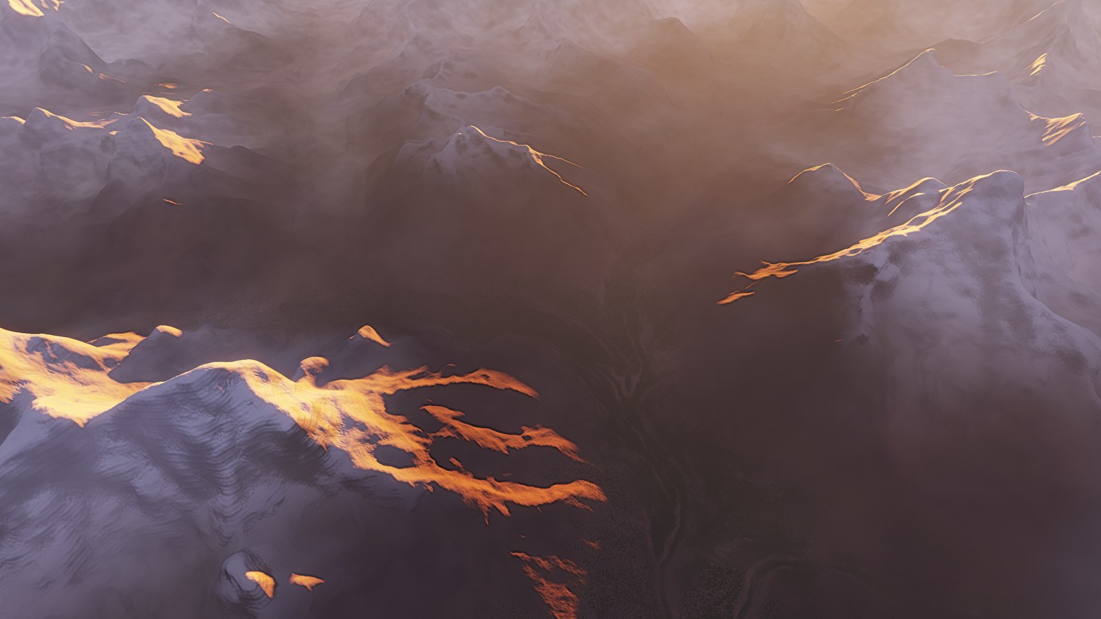
G4, clouds off). Measured GLO-30 relief under the mesh.Levels
One hierarchy. Levels 2 to 9 are stored on disk; 0 and 1 are reductions of 2; every level above 9 is a fixed function of the L9 tile above it. A tile is 512 samples plus a four-texel apron, and the texel size halves per level from 19.5 km at L0.
| Band | Levels | Texel | Source |
|---|---|---|---|
| Derived | L0–L1 | 20 km, 10 km | reductions of L2 |
| Stored | L2–L9 | 5 km … 38 m | GLO-30/GLO-90 blocks; GEBCO through L6 |
| Near | L10 | 19 m | bilinear reconstruction of L9, no invented relief |
| Landform | L11–L13 | 9.5 m … 2.4 m | reconstruction plus accumulated residual bands |
| Grain | L14–L15 | 1.2 m, 60 cm | two more bands plus fixed rocks and rubble |
| Resolved | L16–L18 | 30 cm … 7.5 cm | resampling of the fixed L15 surface |
The rule that keeps this sane: no generated tile is ever the input to another level. L13 samples the L9 tile directly and adds its bands from L11 up; L14 samples the same L9 tile and adds one more. Detail never feeds back into the source, and siblings agree across their shared edge because they read the same ancestor at the same coordinates.
Tiles on the GPU
A resident tile is a 448-byte slot in a table the shaders read by address. Inside a tile every position is expressed in the tile’s own tangent frame — origin at the datum point under the tile centre, camera-relative, refreshed from f64 each frame — so nothing the size of the planet radius is ever subtracted per pixel:
Local tileLocal(uint slot, vec3 p) {
    vec3 q  = p - s.originRel;
    float qn = dot(q, s.n), q1 = dot(q, s.e1), q2 = dot(q, s.e2);
    float rq = FRAME.radius + qn;
    float t2 = q1 * q1 + q2 * q2;
    l.xy = vec2(q1, q2) / rq;                              // tangent-plane coordinates
    l.h  = qn + t2 / (sqrt(t2 + rq * rq) + rq);            // height above datum, cancellation-free
}
Tangent-plane coordinates become texel coordinates through a per-tile cubic (polyU,
polyV, nine terms each, fitted on the CPU) from L5 up, or the exact f32 chart at the
coarsest levels, where a 0.3 m chart error is a thousandth of a texel. The inverse — texel to tangent
plane, which the mesh needs to place corners — starts from a precomputed inverse cubic
and runs three Newton steps on the forward map, so both sides agree on where a texel is
even where the fit is slightly off.
Height reads are explicit. Hardware filtering can quantise interpolation weights to eight bits, which on steep native terrain is centimetres to metres, so the four texels are gathered and interpolated in full precision. At the native level, mixed land/water cells reconstruct a continuous coastline from the binary water mask with a cubic, rather than rendering the nearest-texel waterline.
Level selection is a function of ray distance alone:
float lc = log2(texel0 / (t * FRAME.pixelAngle));  // continuous lod: texel per pixel
uint  L  = uint(clamp(ceil(lc), 0.0, finestLevel));  // the finer of the two blended levels
float w  = clamp(lc - (L - 1.0), 0.0, 1.0) * fade;  // weight of L over its parent
surfaceHeight then walks the parent chain: weight w on this slot (times a spatial
factor that fades a 16-texel band at the tile edge toward the parent, with shared corner
minima so both sides of an edge interpolate identical weights), the remainder on the
parent with the parent’s own arrival fade, until a weight reaches one or the root. The
blended surface is continuous along the ray and across tiles — with one known exception,
below.
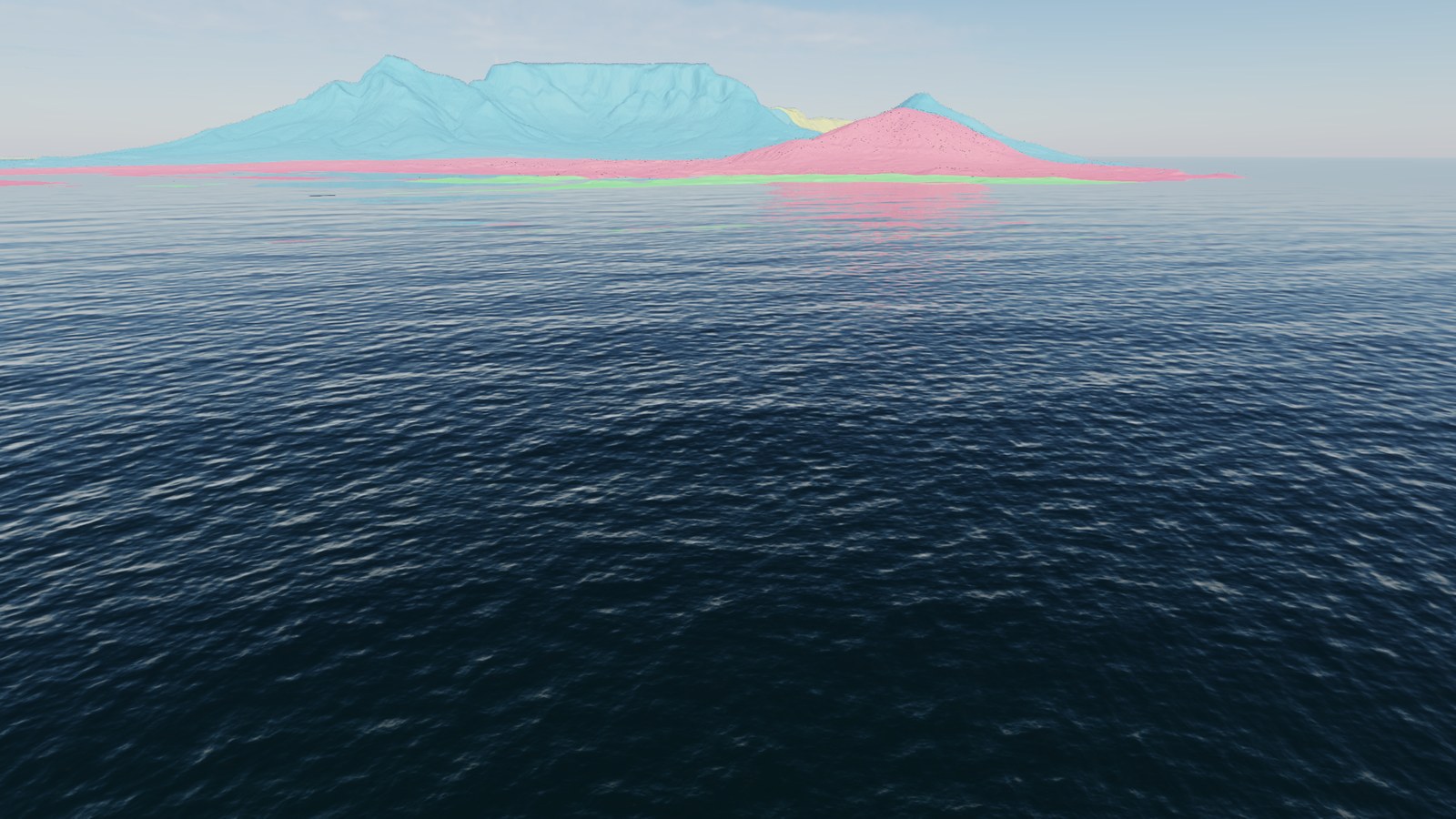
G5), tinted by level. Rings at constant distance crowd toward the horizon.The mesh
There is no cut distance and no far-field ray march. One rasterised concurrent binary tree of bisectors over the cube’s twelve base triangles (each face split on its diagonal) owns every terrain pixel from the whole-planet view to the contact surface. The sky and the ocean are settled afterwards from what the mesh left.
A bisector is 160 bytes in a pool of 2²² entries: a 64-bit LEB path and depth, three corners as 30-bit fixed-point face coordinates, three neighbour indices, the same again for the state the current iteration commits, and this frame’s camera-relative corner positions. Fixed point matters: the midpoint of a hypotenuse is an exact integer to depth 58, so the mesh is conforming by construction and never by epsilon.
The update is one compute shader dispatched in stages, four iterations when splits are pending and one when the frame is quiet:
EVAL        corner positions, screen measure, draw flag (every entry at iteration 0, dirty ones after)
DECIDE      each leaf's split / merge wish; a split wish is pushed to the twin across the hypotenuse
RESOLVE     a split executes when the twin is at the same depth and also splitting (or absent);
            a merge when the four leaves around the shared vertex are two sibling pairs that all want it
RESERVE     leaders turn allocation ranks into pool indices through a sum tree over the free bits
NEIGHBOURS  every survivor computes its next corners, path and neighbours from the old state
COMMIT      next state becomes current; free-bit updates; counters
REDUCE      rebuild the sum tree
FINISH      evaluate the entries created this frame; compact drawable leaves into the indirect draw list
Every pool sweep is an indirect dispatch over the allocated prefix of the pool — free entries are handed out lowest-index first, so a high-water mark bounds the work and an idle pool costs nothing beyond its occupancy.
The split criterion is the interpolation residual: the screen distance, in pixels, between the true surface point at the hypotenuse midpoint and the chord’s midpoint. Split when it exceeds 0.5 px (or when the longest screen edge passes a cap of 24 px, so fragments stay well behaved), merge with hysteresis when the parent would measure under 0.6 of both. The two leg midpoints are checked too, so a crest between vertices that the hypotenuse misses is still caught — that is what keeps silhouettes from showing the far side.
float residualPx(vec3 pm, vec3 pb, vec3 pc) {
    vec3 chord = 0.5 * (pb + pc);
    return length(projectCurrent(pm).xy - projectCurrent(chord).xy);
}
// DECIDE, the gist:
bool split = draw && depth < depthCap
    && (edgePx > edgeTarget(pa, pb, pc)
        || max(residPx, residLegs) > residualTarget(pa, pb, pc));
Two refinements on the targets. The edge cap grows from 24 to 48 px between 5 and 20 km, because far triangles that are also large on screen are fine; and grazing triangles get a target up to 25% tighter, blended in over 2–5 km, because at a grazing angle a small height error exposes a different distant ridge. The depth cap is a function of the finest resident level at the triangle’s nearest corner — children never get finer than a quarter of the texel that actually exists.
Corner evaluation is the dominant cost: six surface evaluations per leaf, each walking the tile chain. Three things keep it affordable. A corner on a cube edge is evaluated on the lower-numbered face from both sides, so shared corners are bit-identical. The level blend depends on distance and distance depends on the height, so evaluation runs two passes — but the second pass reuses the tile walk when the refined distance selects the same level, and caches the first two ancestor height samples (measured: 46% fewer height fetches, 20% faster at eye height). And a decision is cached across the iterations of a frame for leaves whose geometry did not change.
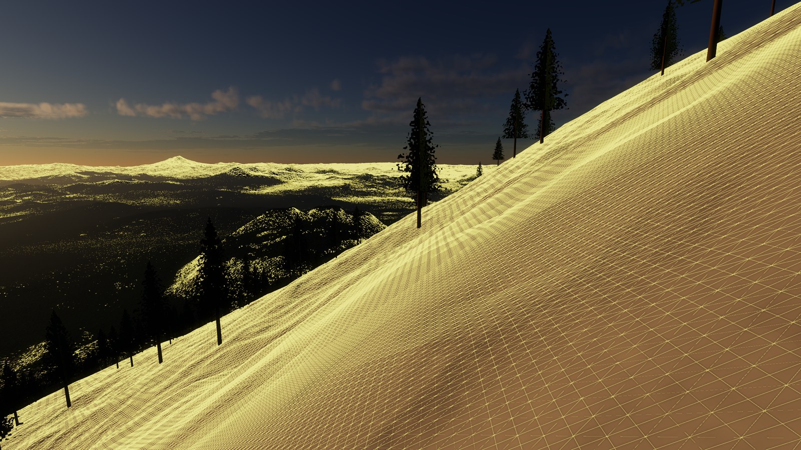
P2), wireframe. About 1.75 million leaves at this kind of view.Publishing a fragment. The fragment stage does not shade. It resolves the fragment’s
tile and texel (fragments past their triangle’s own face are re-addressed on the face
that owns them — clamping to the edge picked the wrong tile and a normal in the wrong
frame), reads the blended surface height, and packs the hit record. One rule here took a
while to get right: the published position follows the surface, not the chord, when
they differ. A coarse triangle seen from orbit is a chord kilometres above a valley at
the limb; lighting, aerial perspective and the ocean must not see that. So if the chord’s
radial altitude and the surface height disagree by more than a metre (or 0.01% of the
distance), the hit is moved to the ray’s intersection with the R + surfaceH shell. The
move is bounded to 10% of the fragment’s own distance and rejected rather than clamped
beyond that: at grazing incidence the intersection is ill-conditioned, and a metres-scale
height correction became kilometres of range — a visible line across the horizon we
carried for a while under the name HORIZ-01.
Horizon cull. A triangle whose three corners’ lines of sight all pass below the datum is dropped before it refines. The datum is a conservative occluder — a summit past the datum horizon still has a clear line of sight and survives — so distant ranges are untouched and only what the planet’s own bulge hides can go. Leaves fell 45% at G5 (100 m over a coast), 13% at 2.6 km near Shasta, 44% at orbit; five of six test views were exact null-diffs. Terrain-occluded mesh is not culled at all; that would need real occlusion.
Streaming
The wanted set is a breadth-first walk of the six face roots, culled by horizon and frustum, emitting every tile whose level is needed somewhere on screen with its ancestors. Priority is screen error — texel over footprint — scaled by where the tile sits in the frame:
let near = (dist - bounding_radius).max(1.0);
let footprint = near * pixel_angle;
let axis = (rel / dist).dot(fwd).clamp(0.0, 1.0) as f32;
let view = 0.5 + 0.5 * axis * axis;          // on the view axis: 2x the edge of frame
let error = (texel / footprint) as f32 * view;
let target = (level_texel_size(radius, 0) / footprint).log2().ceil();
Breadth first, so the 700-tile cap trims the finest levels, which the mesh can serve from their parents; a depth-first cut would drop whole areas. A missing fine tile uses a coarser resident surface; combined demand including parent chains is limited to 75% of the 1,024 slots, the rest holding transition and revisit tiles. Arrivals fade in over 0.5 s against their parent. Completions are handed back in the renderer’s current priority order, not arrival order, so after a fast turn the view being looked at fills first.
The DEM oracle is a worker pool over a shared block cache: sixteen tiles share an 8 MB block and the wanted set asks for neighbours together, so blocks are decoded once and a block another worker is loading is waited for rather than loaded twice.
Same-slot replacement keeps the displayed payload on one of 64 reserved physical pages and cross-fades to the new one over 1.5 s; heights, normals, materials, the CPU ground query and history reprojection all read the same blend.
The feed envelope makes source latency visible. Supply is measured per feed class (derived, stored, amplified) as tiles per second in one-second buckets, counted only while that class has a backlog. Demand is tiles per metre of lateral travel, from the same level rule the walk uses:
/// Tiles of `level` newly wanted per metre of lateral travel at `clearance` above ground.
pub fn tiles_per_metre(radius: f64, level: u8, clearance: f64, pixel_angle: f64) -> f64 {
    let range = 2.0 * level_texel_size(radius, level) / pixel_angle;   // where the level is wanted
    if range <= clearance { return 0.0; }
    let ground_radius = (range * range - clearance * clearance).sqrt();
    let width = 512.0 * level_texel_size(radius, level);
    2.0 * ground_radius / (width * width)    // the disc sweeps 2 g square metres per metre
}
Sustainable lateral speed is supply over demand for the binding class. Bounded flight (off by default) caps manual speed at 75% of that; unbounded flight shows the same numbers and an OUTRUNNING TERRAIN lamp.
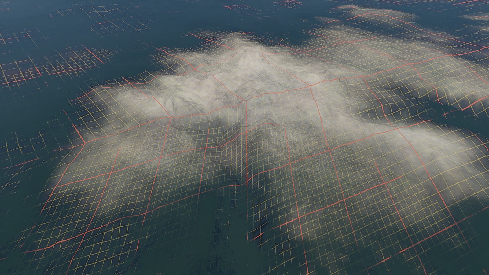
P2a, --tile-grid): tile boundaries in red, the 64-texel grid in yellow. Tiles halve in size as the level rises toward the camera.Above the data
L9 is 38 m. On the ground, a 38 m texel is a smooth blanket, and the detail below it has to be invented. The approach is a real-time approximation to multi-scale erosion residuals, informed by Schott et al. 2024, Terrain Amplification using Multi-scale Erosion (doi 10.1145/3658200): retain the measured low frequencies, add bounded residuals at each finer scale, conditioned by what the coarse surface says about the ground. It is deterministic procedural residuals, not that paper’s erosion solver.
For every texel of a fine tile at level L ≥ 11:
h0, gradient, concavity  <- the L9 ancestor, monotone-cubic reconstruction (bounded by its 4 samples)
region                   <- a 20 km field sampled on the L9 lattice, so descendants can't move it
climate                  <- temperature (lapse-corrected), precipitation at this direction
detail = 0
for level in 11 ..= min(L, 15):
    lambda = 3 texels of `level`
    amp    = 0.10 * lambda * slope_weight * (1 + 0.35 * curvature) * (0.82 + 0.42 * wet)
    amp    = min(amp, 0.30 * lambda)                    # never more than 30% of wavelength
    band   = noise at lambda, shaped by concavity (ridged on convex, valleys on concave)
    on wet, steep, warm slopes: replace with gully noise sampled along the fall line   (level <= 13)
    on cold or dry concave toes at moderate slope: damp toward talus                   (level >= 12)
    on steep faces with the regional strata control: blend toward terraces with fixed
        world-space bedding phase and a six-texel period                               (level <= 13)
    detail += clamp(band, -cap, cap)
if L >= 13: detail += rocks(dir)       # hashed 3D cells on the datum, 35% occupied, accepted once
h = h0 + dry * detail                  # dry fades to 0 across the reconstructed shoreline
Measured water receives nothing at any level; the stored water mask is binary but the shoreline is the reconstructed contour, and land detail fades before its water half. Rocks are placed by hashing fixed 3D cells on the datum sphere and accepting each against a suitability evaluated once at its centre on the L9 surface, so a rock keeps its position, radius and height from L13 to L18 and neighbouring tiles agree without stacking. L16–L18 add no new frequencies: they resample the fixed L15 surface, and material normals and roughness carry the centimetres.
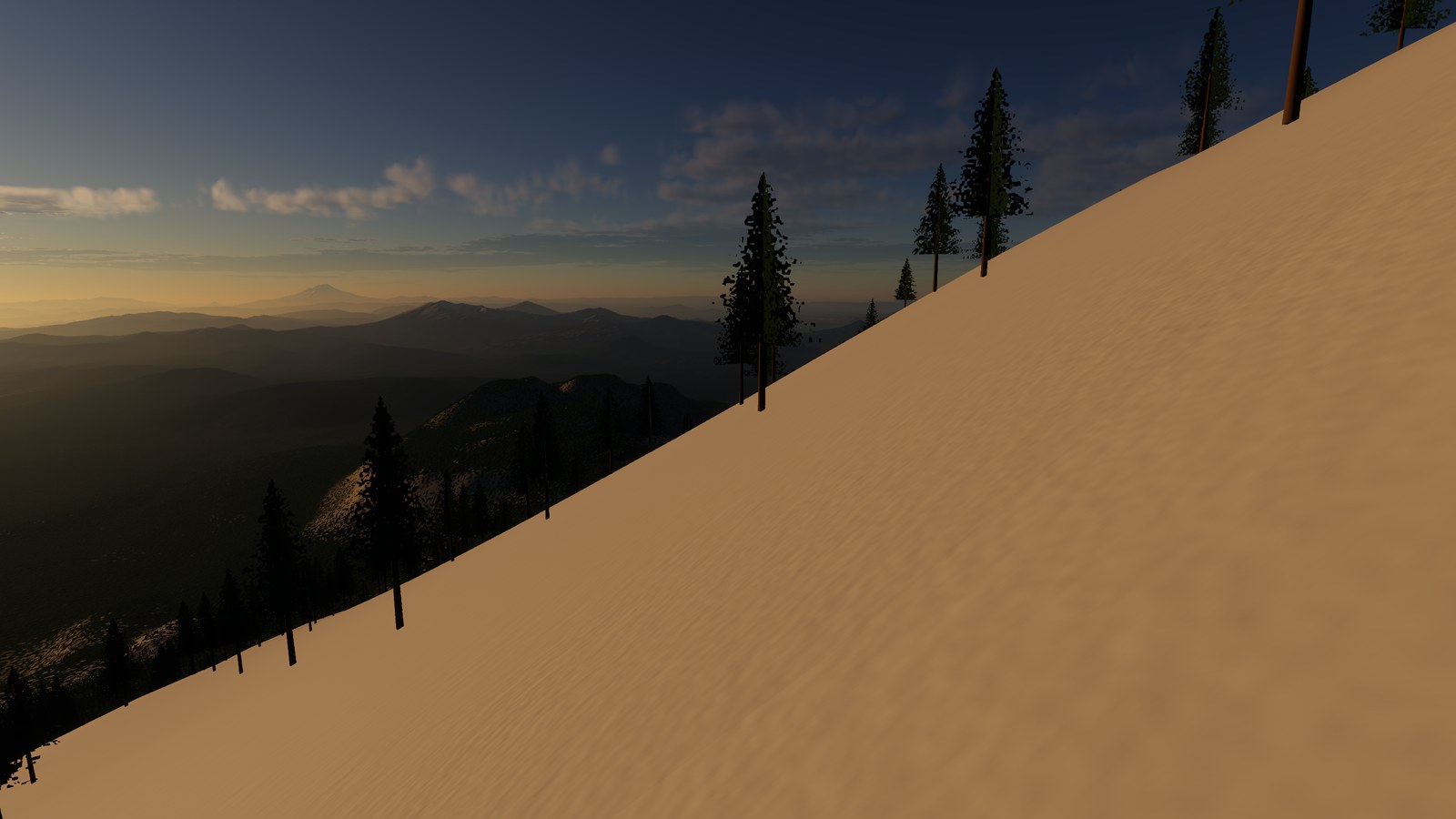
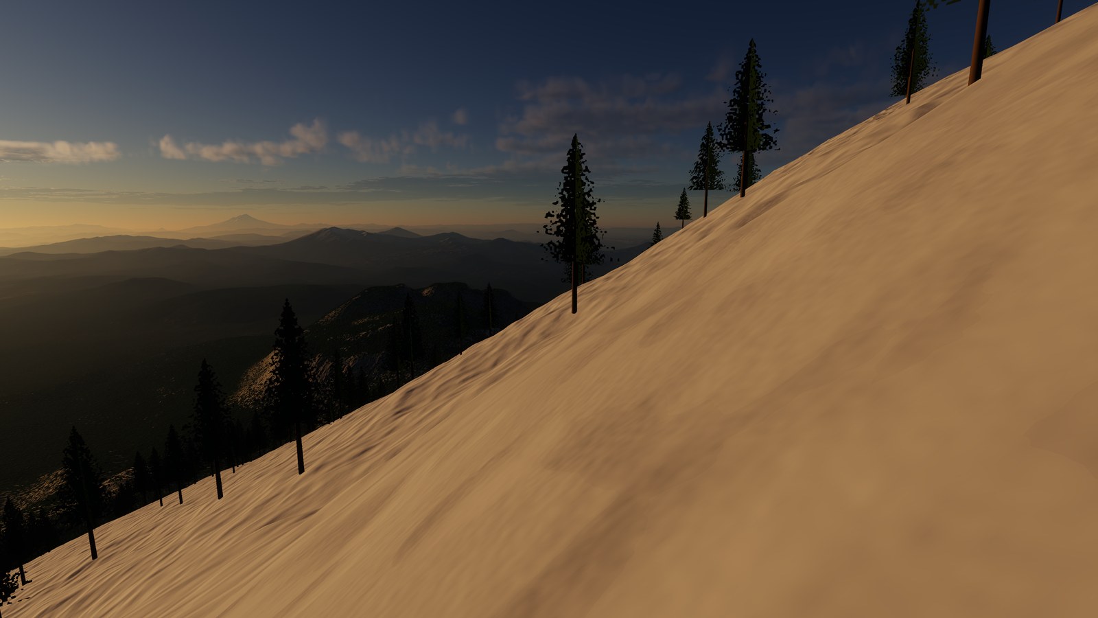
P2). Left: the finest level capped at L10 — the measured surface, reconstructed. Right: the full stack to L18.One control sits over the top of this. The mesh’s decision pass checks fine split candidates against the L14 surface; splits required only by L15+ are counted, and each frame with any of them attenuates a global fine-detail gain by 20%, snapping the tail to zero. At zero gain the geometry stops at L14 and the finer levels live in the materials. The gain holds its last value for the renderer’s lifetime, so a settled camera does not pump between refining and attenuating. It is one global value, not a per-tile quality controller, and the owner chose to keep actual L11–L14 relief and judge its cost by frame time rather than by leaf count.
What is still open
- HORIZ-01, the ring version. Level selection from ray distance makes a level
boundary a ring at constant
t. From a low camera over flat ground the ring projects to a horizontal line, and the blended surface is not continuous across far level boundaries — the step is in the depth and normal buffers, not only in shading. - Occlusion. Only the datum culls. At a grazing ground pose two thirds of the leaves are behind terrain and cover almost no pixels.
- Readiness in flight. A settled hold measures the renderer with its hardest customer absent. Descent has been flown pop-free on the historical route; lateral flight and turning at speed against fresh source are still under review, and the feed has not always been ahead.
- Cold settling. Whole-scene teleports take several seconds to settle even when the fine ground is ready sooner.
Next: the atmosphere — the LUTs, the aerosol, and what the sky does to the ground.