Atmosphere: Air Between the Camera and Everything
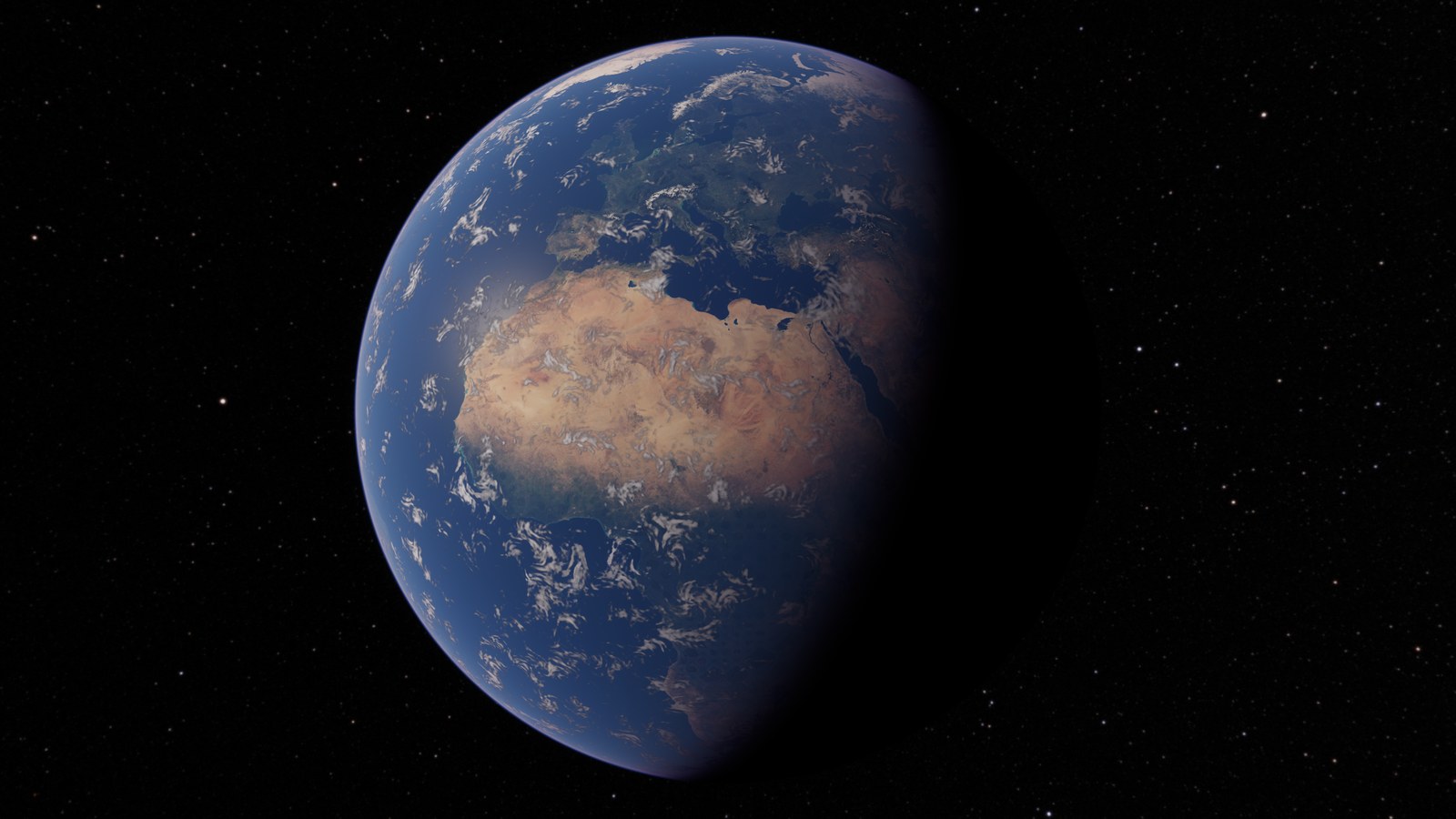
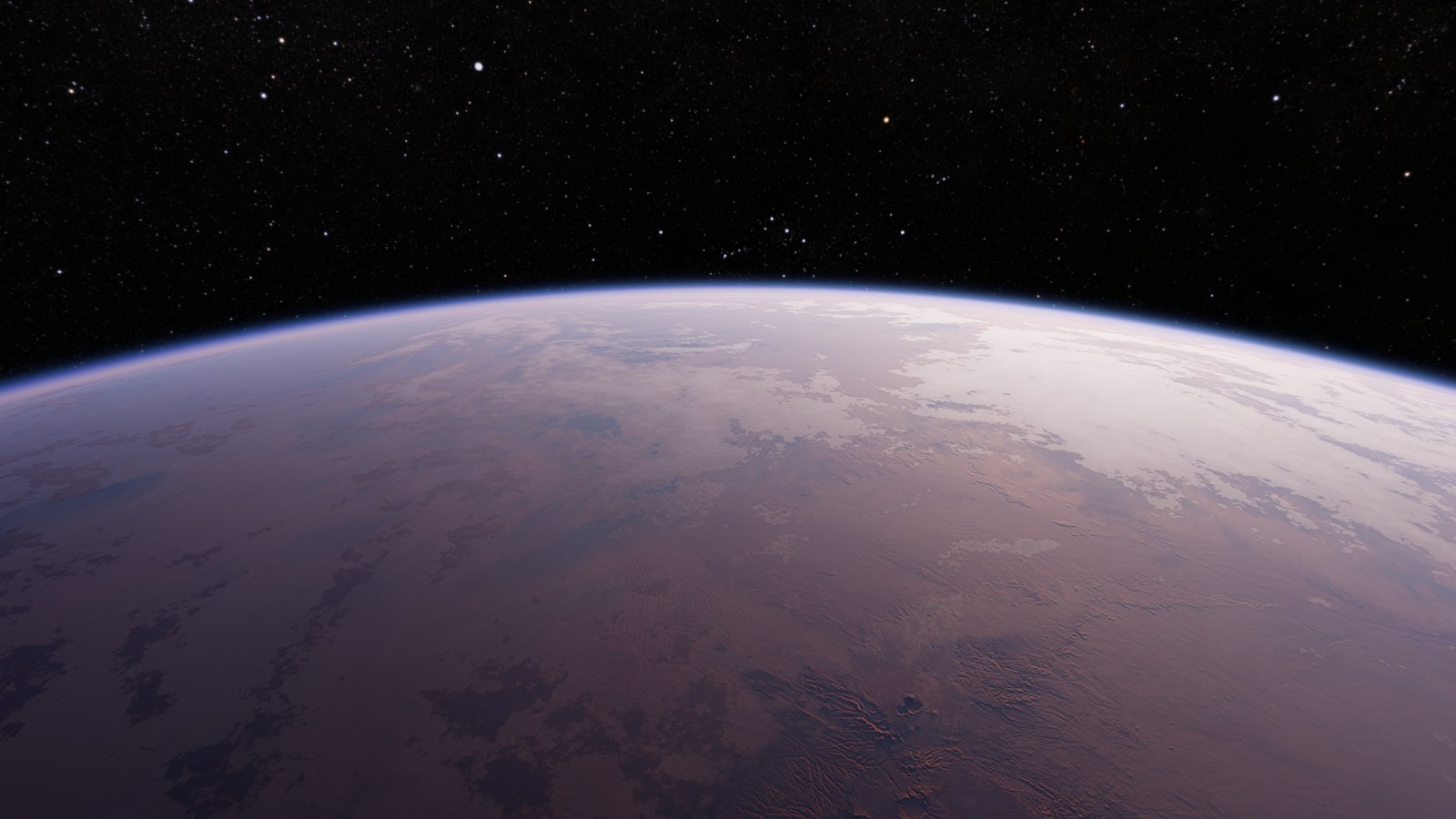
Every pixel in Magic is seen through air, from a full-disc limb to a hazy coast at eye height. The atmosphere is one participating medium — Rayleigh, ozone, and three aerosol populations — integrated by the same functions everywhere, with lookup tables where the integral is a function of few variables and a per-pixel march where it is not. This post is the medium, the tables, the way aerial perspective is reconstructed for a camera that can be anywhere, the aerosol, the bodies in the sky, and surface lighting.
The medium
The model follows Hillaire 2020 (A Scalable and Production Ready Sky and Atmosphere
Rendering Technique), with two additions to the medium. Per height h in metres:
void medium(float h, out vec3 scattering, out vec3 extinction, ...) {
    float rayleigh   = exp(-h / ATMO.rayleighScaleHeight);                        // 8 km
    float background = exp(-h / ATMO.mieScaleHeight);                             // free troposphere, 8 km
    float elevated   = ATMO.elevatedFraction                                       // stratospheric layer
                     * exp(-0.5 * pow((h - ATMO.elevatedCentre) / ATMO.elevatedWidth, 2.0));   // 20 km +- 4 km
    float haze       = exp(-max(h - ATMO.hazeMixedHeight, 0.0) / ATMO.hazeScaleHeight);    // boundary layer, 1 km
    float ozone      = max(0.0, 1.0 - abs(h - ATMO.ozoneCentreHeight) / ATMO.ozoneHalfWidth);  // 25 km +- 15 km
    vec3 sR = ATMO.rayleighScattering * rayleigh;
    vec3 sM = ATMO.mieScattering * (background + elevated);
    vec3 sH = ATMO.hazeScattering * haze;
    vec3 aM = ATMO.mieAbsorption * (background + elevated) + ATMO.hazeAbsorption * haze;
    vec3 aO = ATMO.ozoneAbsorption * ozone;
    scattering = (sR + sM + sH) * 1e3;                 // per km, the LUT domain
    extinction = (sR + sM + sH + aM + aO) * 1e3;
}
The Rayleigh triple is Bruneton’s, (5.802, 13.558, 33.1) × 10⁻⁶ m⁻¹, sampled at 680,
550 and 440 nm. The dry background aerosol is the OPAC free-troposphere value, optical
depth 0.013 at 550 nm above 2 km; Hillaire’s single 1.2 km Mie profile put a quarter of
that aloft and had no boundary layer, so the boundary layer is now its own term. The
elevated layer is the stratospheric sulfate background at optical depth 0.005. The sun
is 120,000 lux, slightly warm across the channels; everything is in nits and lux until
the exposure pass.
The tables
Four LUTs, three of which are Hillaire’s. What is stored in them is the one choice worth explaining.
| LUT | Size | Rebuilt |
|---|---|---|
| Transmittance | 256 × 64, 80 steps | when parameters or humidity change |
| Multiple scattering | 32 × 32, 64 directions × 20 steps | same |
| Receiver irradiance | 64 × 32 | same |
| Sky-view | 192 × 108 × 8 layers, 48 steps | every frame, from camera height and the two lights |
| Aerial-perspective froxels | 32 × 32 × 32 × 9 volumes | every frame |
The multiple-scattering table is the isotropic closure: for a (sun zenith, altitude) pair, integrate single scattering over 64 Fibonacci directions, and also the fraction of light that scatters again, then sum the geometric series.
sL[k] = res.isotropicSource / 64.0;    // directional average of the source
sF[k] = res.multiScatAs1 / 64.0;       // fraction scattered once more
// ...reduce over the workgroup...
vec3 ms = L / max(vec3(1.0) - F, vec3(1e-4));   // all orders at once
The sky-view and froxel tables store unphased transport weights, not radiance. Each texel holds four RGB weights per light — Rayleigh, background aerosol, haze, multiple — at unit illuminance. The phase function is applied at the pixel:
vec3 skyViewLuminance(vec3 d, uint layer) {
    vec3 ld = layer == 0u ? FRAME.sunDir : FRAME.moonDir;
    return illuminance * ( atmosphereDirectSource(d, ld, angularRadius,
                               weightRayleigh, weightMie, weightHaze)   // phases applied here
                         + weightMultiple );
}
That is why the sun’s aureole is sharp: a 192 × 108 table cannot resolve a forward Mie lobe, but it does not need to. The lobe is evaluated per pixel against the actual sun direction, and the phase itself is filtered over the sun’s disc plus the pixel footprint with a two-ring quadrature, so it neither aliases nor blurs.
Heights along a ray use the same cancellation-free form the rest of the engine does:
// Height above the datum at distance t along a ray from height h0 with cos a = -d.up.
float rayHeightAt(float h0, float cosA, float t) {
    float rh = FRAME.radius + h0;
    float r  = sqrt(max(rh * rh + t * t - 2.0 * t * rh * cosA, 0.0));
    return (h0 * (2.0 * FRAME.radius + h0) + t * t - 2.0 * t * rh * cosA) / (r + FRAME.radius);
}
Inside the LUT integrators positions are planet-centred in kilometres, where f32 is fine; the render frame never holds a planet-centred vector.
Aerial perspective for a camera that can be anywhere
The froxel volume is camera-space, 32 × 32 × 32, slice s ending at (s/32)² ×
range, with the range set per frame to 1.3 × horizon distance + 20 km (at least
32 km). That is enough from the ground and from cruise. It is wrong in three places, and
atmosphereSegment handles each:
- Beyond the froxel range, or above 95 km where the camera is leaving the air, the segment is marched per pixel (32 steps sun, 12 moon), blended in over the last 10% of the range.
- Near the horizon. A froxel column is clipped at the ground, and the four angular neighbours a pixel interpolates between do not share an endpoint. So the reconstruction is done at a common endpoint altitude, not a common ray distance: each neighbour’s ray is intersected with the shell at the pixel’s endpoint height, that neighbour’s column is sampled at its own distance, and the four are then blended. Within one froxel of the tangent direction — where that intersection is singular — the march takes over.
- From space, the whole sky is a per-pixel march (40 steps) and the sky-view table is not consulted.
AtmosphereSegment atmosphereSegment(uvec2 pix, vec3 d, float distance) {
    float direct = max(smoothstep(0.9 * range, range, distance),
                       smoothstep(top - 5000.0, top, FRAME.altitude));
    // ...plus 1.0 within one froxel of the camera-horizon tangent...
    if (direct < 1.0) seg = froxelSegment(pix, d, distance);      // reconstruct at endpoint altitude
    if (direct > 0.0) seg = mix(seg, marchAtmosphereSegment(d, distance), direct);
    return seg;   // color = color * seg.transmittance + seg.luminance
}
The result is one contract — transmittance and in-scattered luminance over a segment — used by terrain, ocean, clouds and the vegetation alike, from any altitude.
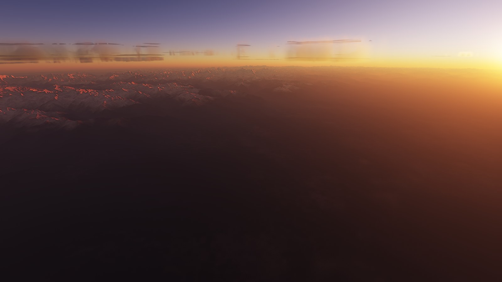
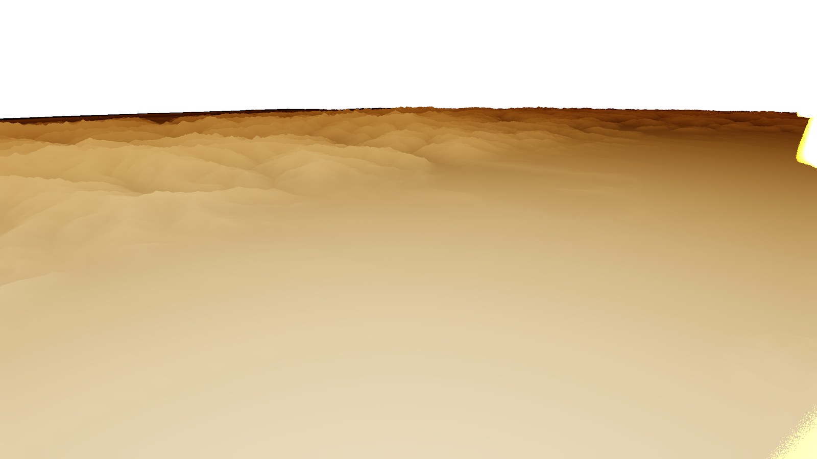
A1). Right: the transmittance the aerial perspective multiplies in (--debug-view 6).The aerosol
The background medium alone is about 22 × 10⁻⁶ m⁻¹ at sea level — a Koschmieder visual range of 178 km. No real day is that clear, so distant ridges arrived at full contrast and distance never softened. The boundary-layer haze fixes that, and it is driven by the weather rather than a constant:
sigma_haze(h) = haze(RH) * exp(-h / 1 km)
haze(RH)      = 30e-6 * clamp((1 - RH)^-0.6, 1, 6)        Hänel growth, capped short of fog
Relative humidity comes from the weather field under the camera, which traces to measured WorldClim rain: Vatnajökull sits at 0.91, the 45 E anchor at 0.25, with nothing tuned per site. Visual range across the catalogue views runs 27–68 km, against 20–60 km on a real clear day.
Both aerosol terms are RGB. Each coefficient is its 550 nm value spread over the channels
by Ångström’s law, sigma(λ) = sigma(550) (λ/550)^-α, on the same three wavelengths
the Rayleigh triple is sampled at — recovered from the table itself, since
13.558 × (550/680)⁴ = 5.802. The haze exponent falls with humidity because a swollen
particle scatters more neutrally: 1.30 dry, 0.63 at Vatnajökull. Scattering and absorption
carry different exponents (1.5 for absorption, a continental mix), which gives the aerosol
a wavelength-dependent single-scattering albedo and lets thick humid haze brown a horizon
instead of only bluing it. Over twelve views from 15,000 km to eye height the effect is
under 0.35 of 255 above 400 km and 2–4 levels of red at eye height — a ground-level
effect, as it should be, since a near-horizontal ray from 10 km crosses no boundary layer.
Phase functions are offline Lorenz–Mie tables for two populations (1,025 angles on a
θ = π u² grid, dense at the forward peak), with a per-sample mode after Bennett that
evaluates the Jendersie–d’Eon approximate-Mie fit at a droplet diameter that changes
with the layer and grows with humidity. Cornette–Shanks and Klein–Nishina exist for
comparison.
Limits: the haze is horizontally uniform, sampled at the camera. The transmittance and multiple-scattering tables are functions of height and sun angle only and cannot carry a position, so flying from a dry region into a wet one changes the whole sky at once rather than showing a humid valley ahead. That needs a near froxel volume and is not built.
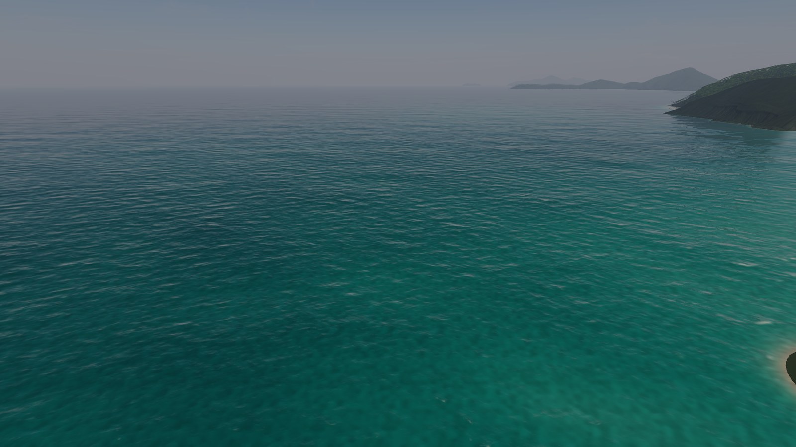
E3), RH 0.95: the wettest and haziest of the catalogue views.Bodies
The sun disc has per-channel linear limb darkening — stronger in blue, so the limb comes out warmer — normalised so the disc’s mean radiance is the physical one whatever size is drawn. The moon is a phased sphere with a Lommel–Seeliger regolith term (the lit limb stays bright and the full moon flat), an opposition surge over the last eight degrees toward full, earthshine on the night side and an albedo texture; its total light is the physical illuminance for the current phase. The star field is the NASA celestial panorama, rotated by sidereal time, occluded by the planet and attenuated by the air. In space it is given a bounded display gain so it stays visible beside a sunlit Earth; the exposure pass subtracts that gain again before metering, so the display response never becomes its own input.
Refraction. Bodies are seen along the refracted ray: lifted and flattened at the
horizon and visible a little past it. A 64 × 256 table (camera height, apparent elevation)
holds the bend, computed once by marching Bouguer’s invariant n r sin z through an
exponential refractivity profile:
// Refractivity n - 1 = 2.77e-4 * exp(-h / 8400 m). Bend accumulates as -(dn/dr)/n * sin z
// per unit arc length, which stays finite through the perigee, so march arc length.
while descending || r < top {
    let sin_z = (k / (n * r)).clamp(0.0, 1.0);
    let cos_z = (1.0 - sin_z * sin_z).max(0.0).sqrt();
    let dn_dr = -(n - 1.0) / SCALE_HEIGHT;
    let ds = (SCALE_HEIGHT * 0.02).max(cos_z * 500.0).min(2000.0);
    bend += (-dn_dr / n) * sin_z * ds;
    // ...step r, turn at the perigee, stop at the ground or the top...
}
A unit test checks the horizontal ray from sea level against the almanac: about 34 arcminutes. A camera above the atmosphere is mapped onto its top by the vacuum invariant.
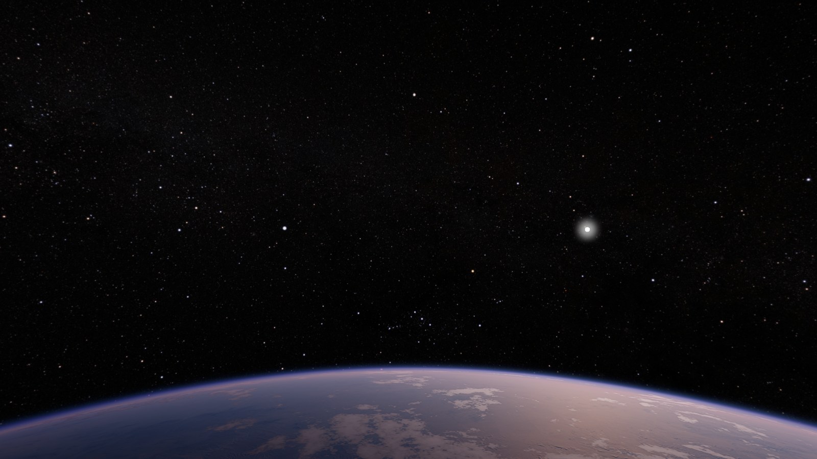
G3).What the sky does to the ground
Surface irradiance is direct sun through the transmittance table times a shadow term, the same for the moon, sky irradiance at the receiver’s height and normal, and a starlight floor:
vec3 surfaceIrradiance(vec3 n, vec3 up, float h, vec2 shadow, float skyVisibility) {
    vec3 sunE  = ATMO.sunIlluminance  * sunTransmittance(h, dot(up, FRAME.sunDir))  * shadow.x * max(dot(n, FRAME.sunDir), 0.0);
    vec3 moonE = vec3(ATMO.moonIlluminance) * sunTransmittance(h, dot(up, FRAME.moonDir)) * shadow.y * max(dot(n, FRAME.moonDir), 0.0);
    vec3 skyE  = receiverSkyIrradiance(n, up, h) * skyVisibility;
    vec3 starE = vec3(ATMO.starlightIlluminance * 0.5) * (0.5 + 0.5 * dot(n, up));
    return sunE + moonE + skyE + starE;
}
sunTransmittance integrates the finite solar disc against the horizon, so the terminator
softens instead of switching. The terrain shadow is a per-pixel ray over the resident
tiles: twelve samples in geometric progression from two receiver texels out to 8 km, each
reading the surface band-limited to its own spacing, with a penumbra from the sun’s
diameter widened by the receiver’s pixel footprint. Fixed midpoint quadrature, not
random phases — a stochastic version produced a noisy band that TAA could not average on
a stationary camera, and removing it cut the frame-to-frame variation of a shadow crop by
91%.
Exposure meters two histograms of the same frame: the whole of it, and the same samples with black space progressively removed as the camera climbs. The host blends the second into the first by the share of the frame it holds, so a planet entering the frame moves the metering target continuously rather than switching source on the frame its last sunlit pixel leaves. Adaptation is asymmetric — a 0.3 s time constant toward a brighter scene, 2.5 s into darkness capped at 1.5 stops per second — so a glance away cannot leave the exposure somewhere the return blows out from. A one-workgroup guard runs over the histogram the current frame just wrote and bounds the applied exposure to within a stop of what this frame asks for; it only ever darkens and needs no readback.
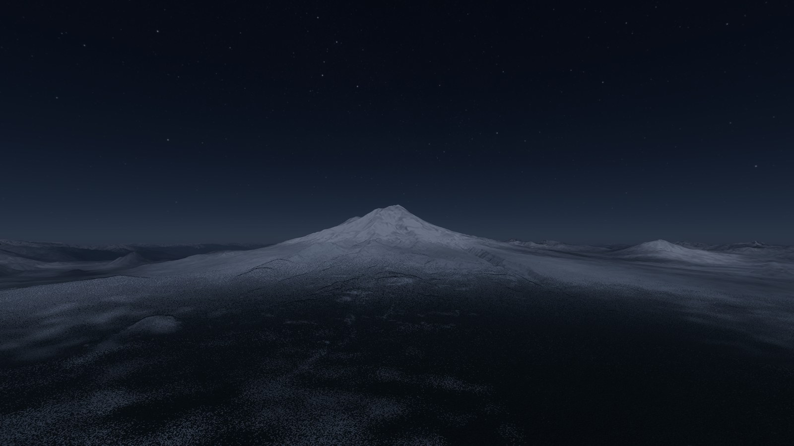
Open
- Positional haze (a near froxel volume that carries fog and humidity where they are).
- Stars are catalogue-derived but on an artistic radiance scale, not radiometric; the moon is not yet a terrain body.
- Long terrain horizons beyond the 8 km shadow ray — horizon maps are designed, not built.
- Clouds are their own system (a weather field, a cloud column, a march, a layer and a statistic) and deserve their own post.